I lasso and I ridge and I don't overfit

Let’s say I want to use a machine learning model to make a prediction, a common example is predicting height, and I have a dataset with many features. Now, a lot of those features have nothing to do with a person’s height, such as their income or hair color, but my model is learning from those features too.

Walter is 5 foot 9 (1.75 meters) because he is a business man with blonde hair, blue eyes, has three children, and likes the color red. Sally is 6 foot 1 because (1.85 meters) because she is a math teacher with red hair, brown eyes,...

The model is overfitting. It is learning the training dataset too specifically and capturing patterns that don’t exist, which makes its predictions on the test set inaccurate because it is struggling to generalize.

Regularization weakens the impact of irrelevant predictors in the dataset. The loss function takes into account how far our predictions are from the true labels. When we minimize the distance between predictions and true labels without considering that some of our data might not be useful for the prediction, the model adjusts its predictions too precisely to the noise.

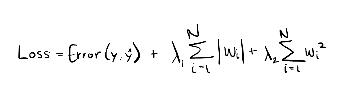
L1 regularization and L2 regularization are applied as an extension of the loss function. A penalty term that penalizes the importance given to features that aren’t relevant to the prediction. The example below is a linear regression problem because the relationship between relevant features can be expressed as a linear combination of features and their coefficients.

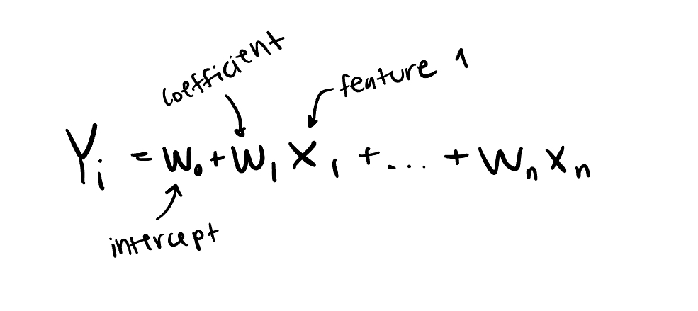
In linear models, the coefficient of each feature is the weight placed on the importance of that feature. More generally, we refer to that number as a parameter, which is the number that any machine learning model adjusts to find the proper weight to apply to each feature. It’s good to know that L1 and L2 Regularization can be applied to prediction problems with non-linear data as well.

In fact, L2 regularization is often used in neural networks. For example, a CNN used to classify images. Applying L2 regularization prevents weights of neurons from getting too large, referred to as weight decay. L1 regularization can be applied as well, but L2 is more common in the case of neural networks because of L1’s tendency to create sparse solutions, but we are getting a bit ahead of ourselves now.

Moving sequentially, let’s start with L1, sometimes referred to as LASSO. Why LASSO? Hold your horses, we will circle back to that shortly.

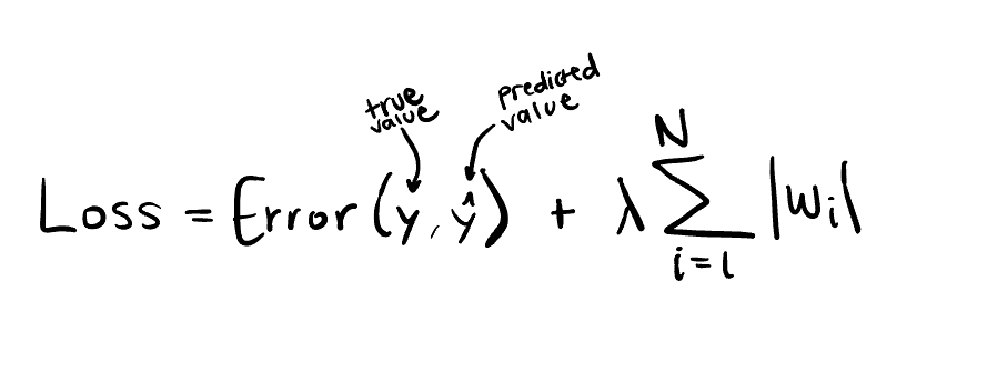
L1 Regularization adds the sum of absolute values of each coefficient as a penalty term to the loss function.

One of its distinctive qualities is that feature selection is built into it, since it completely eradicates the impact of the features that aren’t relevant by pushing their coefficients to exactly 0, which results in a sparse, zero-ful solution. However, it’s important to note that when two features are highly correlated, such as age and weight in our height prediction problem, only one of them stays. So, it’s best to choose the one you want to keep for interpretability reasons before L1 regularization arbitrarily removes one itself.

So why is it called LASSO? Least Absolute Shrinkage and Selection Operator, which refers to its shrinkage of parameters to 0 using the absolute value penalty term and to the resulting feature selection. I was hoping it would be more exciting than that too, maybe something about cowboys.

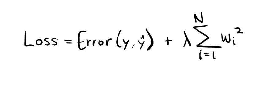
Then, we have L2 regularization, also known as Ridge. I’ll leave you on a cliff hanger for that one too, but don’t get your hopes up. L2 adds the squared value of each coefficient as a penalty term to the loss function.

It shrinks the model’s parameters, but never to zero exactly. It’s useful in scenarios where all features are expected to contribute to the prediction so that none of them get cancelled out. We could say that it sort of handles multicollinearity, which is when two highly correlated variables make it hard to tell which one contributes to the prediction problem more. Unlike L1, which just removes one of the two correlated features, L2 has the coefficients of correlated features influencing the model equally, which affects interpretability since it’s harder to identify the more important one.

So, why Ridge? Well, the term ridge was borrowed from ridge analysis, which studies contours and stuff. Geometrically, when there is a multicollinearity, the graph of the loss function becomes flat where it is normally curved. It becomes unclear which solution is better or worse because there is a flat plane of equally good solutions, a ridge. L2 regularization adds a curved penalty that makes it possible to find a minimum.

Now, you might be wondering who this guy is

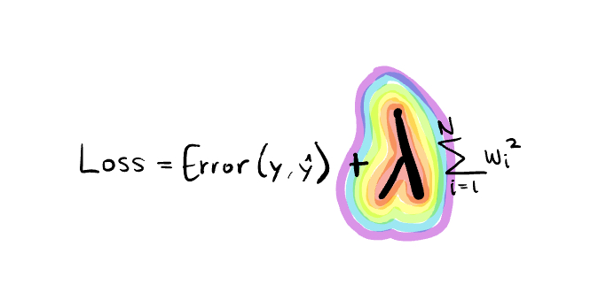
λ (lambda) represents the strength of regularization. With regularization, we are aiming to balance bias (difference between true value and our prediction) and variance (fluctuations in the model’s predictions) to reach generalization. Regularize too much, bias skyrockets, also known as underfitting. Regularize too little, variance does, also known as overfitting. How to choose lambda is outside the subject matter of this article, but simply put, we can test various values and iteratively monitor and adjust it.

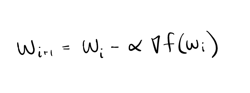
How are we moving the coefficients? Why does L1 go to zero and L2 doesn't? The answer lies within the magical powers of gradient descent. We move in the opposite direction of the derivative of the parameter, which represents the steepest increase of the loss function, in an effort to move toward the minimum of the loss function.

When we take the derivative of the penalty term of L1 regularization, it's always going to be positive or negative 1, so we move towards 0 consistently until we reach it and when we do, the derivative becomes 0 as well, leaving that coefficient at 0.

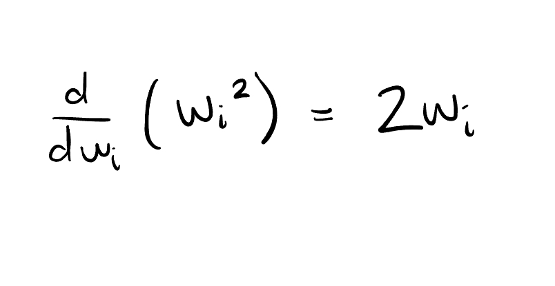
Meanwhile, the gradient of the penalty term in the case of L2 regularization is 2 times the coefficient, so as the coefficient gets smaller, the steps we take towards 0 as we approach it get smaller too.

It’s useful to visualize the difference between the two methods. For L2, we create a circle with a radius of s and for L1 we create a diamond with each corner at ±s. The yellow region is the constraint of how large the parameters can be, bounded by s. The constraint bound s is controlled by λ (lambda). A smaller s is a larger λ, a stronger regularization, and vice versa, so we pick s as we pick λ. The ellipses represent the contour lines of the loss function of linear regression. The optimal answer is touching the edge of the constraint region.

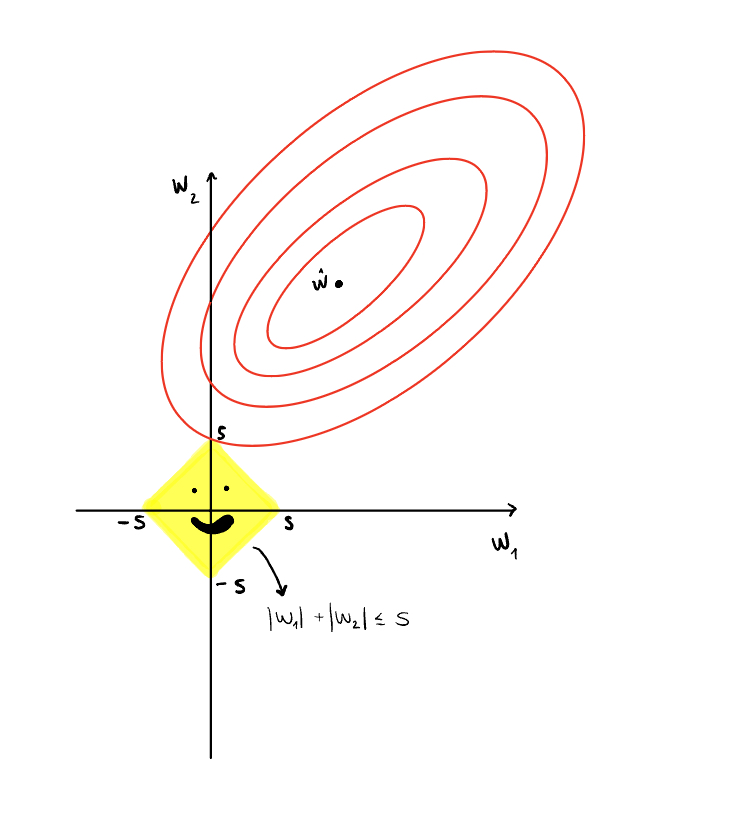
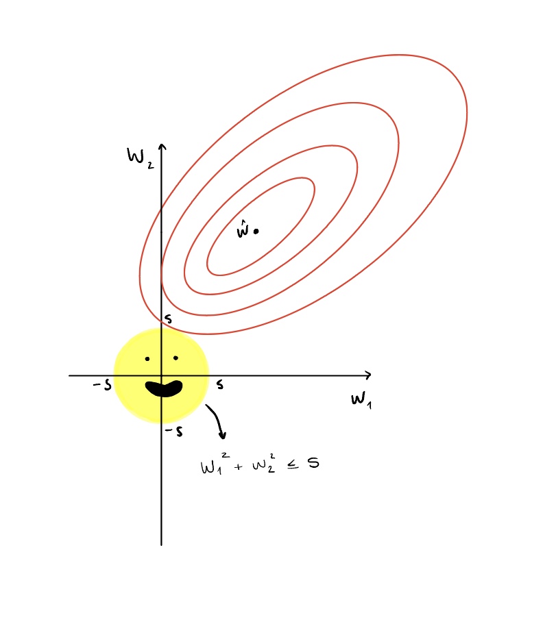
Too far inside and we may start to underfit. Too far outside and we continue to overfit. In reality, the graphs are multidimensional, since there would be more than two features in any prediction problem, but here we just show two, w₁ and w₂, for conceptualization purposes. ŵ is the vector of coefficients that minimize the loss before we apply regularization. We want to just touch the edge of the constraint region with one of the contours because that is the lowest possible loss that satisfies the constraint.

Looking at the L1 visualization, it is more likely for one of the contour lines to hit a corner of the diamond and the feature on that axis to go to 0. Looking at L2, the contour lines can approach 0, but it is highly unlikely that they meet the constraint circle at exactly 0.

Now, another regularization technique that is referred to as Elastic Net is the combination of L1 and L2. Named for its flexibility and adaptability to accommodate to data as a hybrid regularization method.

It provides us with feature selection and stable weights, so some parameters go to zero, but not as many as L1. For correlated features, Elastic Net keeps both and shrinks their coefficients together, as L2 does. It’s like a rounded diamond graph, some features land right at the curved tip, but not many.

So now we know what to do if we have a complex dataset for a prediction task that requires a not-so complex model. We lasso and we ridge and we don’t overfit!

Or, we at least reduce overfitting, since it’s not guaranteed that L1 and L2 regularization cure overfitting every time, they are just one tool. Other regularization techniques not discussed here include Dropout, Early Stopping, Data Augmentation, and Batch Normalization.