Imagine you and a team of people have written a children’s book that ended up being a best-seller. Now, you have all these earnings from book sales flowing in and you want to make sure they are divided evenly amongst the team. You all came up with the title together, you and Emma wrote the story, Emma and Juliette did the illustrations, Aleia was in charge of editing, and so on. You all worked on it in different combinations of teams as well as individually, and some contributions were more valuable than others. So how do you split the earnings fairly?
The Shapley value is a game theory based concept often used in economics. (Game theory is, briefly put, the study of interactions as mathematical models). Let’s say each person who contributed to the book is a player and the project of publishing the book is the game. How it works in game theory is that the contribution of each player is measured so that everyone gets a fair payout based on their contribution. Shapley value is the payout given to each player (2), calculated as their average contribution in all coalitions.
Let’s take a look at a venn diagram (9) and start slowly. Say it was just you and Emma that made the book.
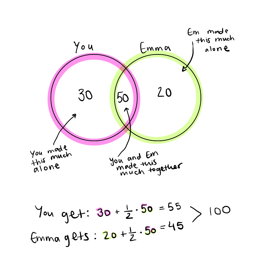
It’s deceptively straightforward. The work you did was worth $30,000, the work Emma did was worth $20,000, and the work you did together was worth $50,000, for a grand total of $100,000 in earnings. So, you made $55,000 based on your individual $30,000 plus $25,000 (half of the $50,000 you made collaborating with Emma) for a total payout of $55,000. She made her individual $20,000 plus $25,000 (the other half of your collaboration’s $50,000) for a total payout of $45,000. Pretty lucrative for a children’s book.
Now, let’s re-imagine that Juliette was on the team too and that the three of you created this book together.
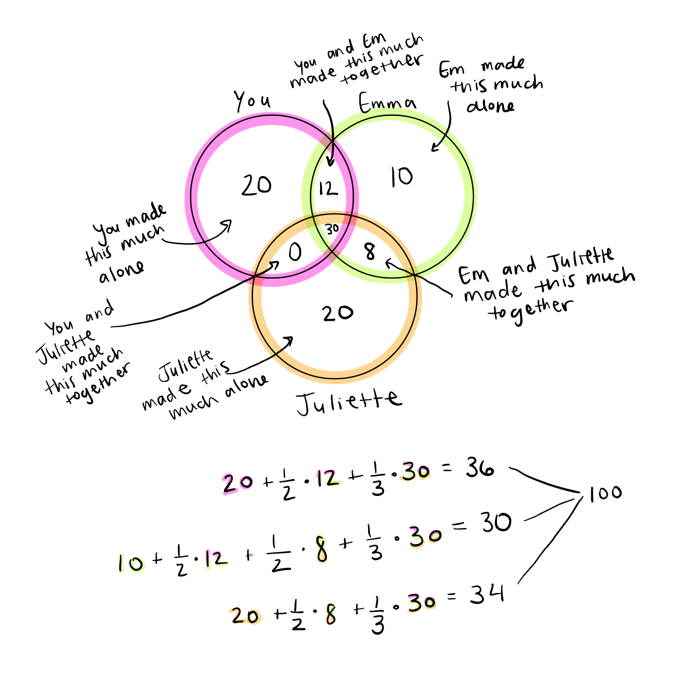
Now, we have to consider not only the work you and Emma did together, but also the work that Emma and Juliette did together, the work you and Juliette did together (in this case none), and the work that all three of you did together. Still, the total is $100,000. Shapley values will always add up to the total earnings.
This is actually when I found out it’s geometrically impossible to do a four-way venn diagram with circles (with ellipses it’s possible). Something about how circles can only intersect at two points which makes it impossible to show all possible intersections of four. Sorry Aleia.
The theory follows also some axioms: Each player contribution must add up to the total (Efficiency), any player who doesn't contribute gets zero (Dummy), players that contribute the same amount get same score (Symmetry) and if we combine two games (like publishing a sequel to our book and adding up how much we earned), the Shapley values also add up (Additive/Linear). Blah blah math.
Here’s a fun fact to ease the weight of carrying all that theory. You might be wondering, where does the name “Shapley” come from? The inventor of Shapley values is none other than Lloyd Shapley. He received a Nobel prize in economic sciences, but for a different theory than the one we are discussing. According to his Wikipedia page, he debated accepting it as he thought that his late father, astronomer Harlow Shapley, deserved it more, but his sons convinced him to accept it.
Moving on. Why is this useful for machine learning?
In machine learning, the Shapley value measures how much a feature contributes to the final prediction. A lot of models have high prediction accuracy, which is cool and all, but ultimately we don’t know why a model made the prediction that it did if we only look at the accuracy. For example, maybe we have a model that is highly accurate at identifying which patients need a certain medication. We calculate Shapley values and look at which features are contributing most to the final prediction and we find that gender is contributing a lot when, from a clinical perspective, gender is not relevant in whether a patient needs this medication. So, not only can we see exactly which features the model thinks are important for the prediction, thus making the model more interpretable, but we can also uncover bias in the predictions.
So how do we implement Shapley values in machine learning models? Let’s say we have trained a model to predict a person’s credit score. We give the model one instance (one person) and it predicts that specific person’s credit score. The task of predicting their credit score is like the game, the features of that single person are the players, and the payout is the prediction for this person minus the baseline prediction across all instances (5).
Note: Shapley value measures the average contribution of a specific feature to the prediction and how much the prediction changes when that feature enters a coalition. Shapley value does not measure the difference in the prediction when we remove that feature from the model.
To calculate Shapley values, we can follow similar reasoning as above with the venn diagrams. However, there will be some differences in logic since now we are working with a machine learning model instead of with book sales. Take a look at this flow chart (1) and start with just two features to include in our credit score prediction model: payment history and amount owed. The box is the model and the letters inside each box are the features used to train the model, starting from the baseline prediction over the whole dataset with no known features. Obviously, we can’t run the model with no features, so we make them unknown rather than removing them.
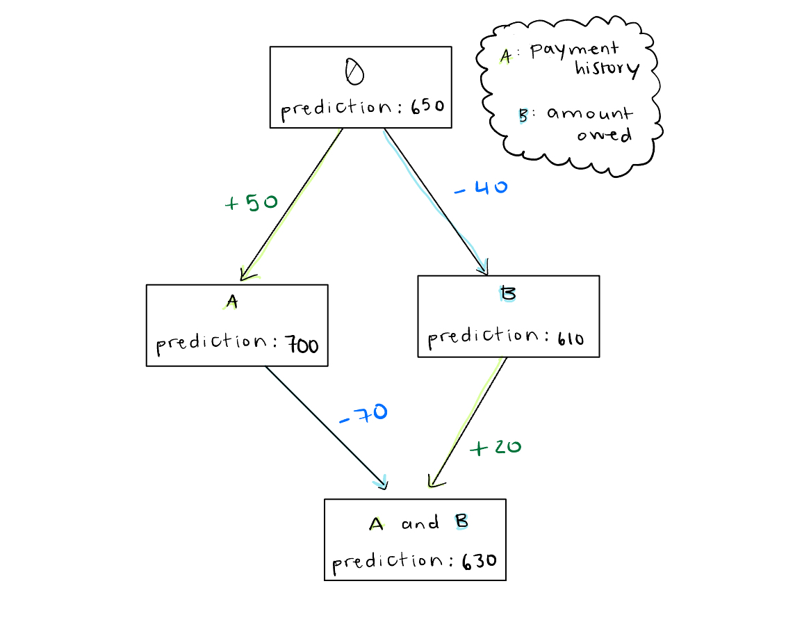
Let’s focus on calculating the Shapley score for feature A. When we first make only A known, the prediction increases by 50 credit score points. Then, when we separately make B known and add A to make a coalition of A and B, the prediction increases by another 20 points.
The reason we half 50, and half 20, then sum them together in the final calculation, as shown below, is because we are summing the averages. When we add feature A first , it is one of two options: AB or BA, and when we add feature A after adding feature B to make a coalition, it is also one of two options: AB or BA.
To calculate the Shapley score for B, we follow the same process. That gives A a Shapley score of 35 and B a Shapley score of -55. Add those up and we get -20 which, if we reference the flow chart above, is exactly what we need to get from the baseline prediction where we started to the final prediction where we ended.

Ok, let’s add another feature: credit history length. I don’t mean to be redundant, but I think it is important to see how exponentially quickly the complexity of calculating the Shapley value grows, even when we just go from two to three features.
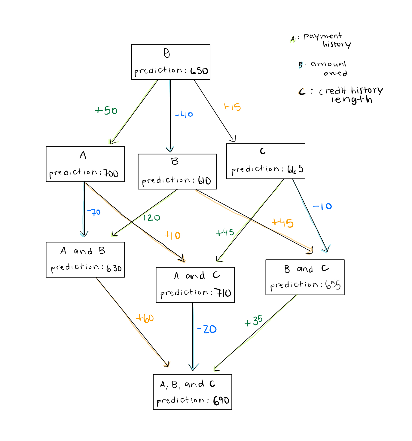
Start with A again. It adds 50 points to the prediction when added first and is two of six possibilities, ACB, ABC, BCA, CBA, BAC, CAB. Then, if we add it after adding B it adds 20 points and is one of 6 coalition possibilities: BA, AB, BC, AC, CB, CA. Or, if we add it after adding C, it adds 45 points and is one of 6 possibilities again. Finally, if we add it after adding B and C, it adds 35 points and is two of six possibilities again. And following that math, feature A has a Shapley value of 39 ⅙. If we look at the arithmetic below, when we add up all the Shapley values, it is once again what we need to add to the baseline prediction to get the final one.
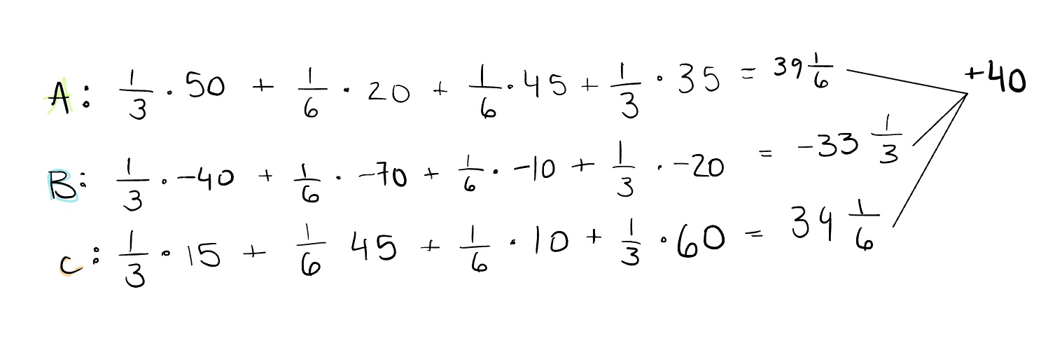
Now, imagine having hundreds of features. By the theory explained above, we would have to retrain the model for each possible combination of features in order to get the Shapley value for each feature. Given that f is the number of features, we would retrain 2f times (1). Sounds a bit computationally complex, and, if we have a lot of features, maybe even infeasible…
Enter SHAP, or SHapley Additive exPlanations. Love the creativity with the capitalization choices here by the way.
SHAP is a way to estimate Shapley values for model interpretation which combines Shapley value theory with various post-hoc interpretation methods (6). It was introduced in this paper by Scott Lundberg and Su-in Lee in 2017 and can be installed as a Python library called shap. The point of SHAP is to explain how the model behaves, not how correct it is, and it’s essentially an approximation of the Shapley value that mitigates the issue of retraining so many times when there are a lot of features to consider.
There are many different SHAP methods which depend on the type of model we are implementing. For example, KernelSHAP can be applied to any model. It combines Shapley value theory with another interpretability mechanism called LIME, which stands for Local Interpretable Model-agnostic Explanation. However, even though it’s pretty common to find it mentioned in discussions about SHAP, the shap Python package doesn’t even use this method because it’s so slow. I suppose what’s most interesting about it is the fact that it’s model agnostic, whereas the rest are specific to the type of model, see: Deep SHAP, Tree SHAP, Linear SHAP, etc.
Another Shapley value based method is ShapleyVIC, or Shapley Variable Importance Cloud (7). SHAP on its own just measures the features of one model, but ShapleyVIC calculates Shapley scores for a number of nearly optimal models (which is relevant to the FAIM framework that I’m exploring for my thesis) and then summarizes the results (8). It’s essentially exploring if feature importance is stable or varies a lot, thus capturing uncertainty in Shapley values across different models. I haven’t really seen it mentioned in SHAP articles and maybe it is very specific to FAIM, but I think exploring uncertainty in anything machine learning related is very important, so I’ve included it here.
Now, I hope we can not only use SHAP to increase interpretability (and potentially mitigate bias) in our machine learning models, but understand a bit more about how it works too.


