
The Iris dataset is one of the earliest datasets used for evaluating machine learning models for classification tasks (1). As someone named Iris, I feel inclined to use this dataset for our opening example.
Now, I want to start slow, so even though there are three species of iris flowers in this dataset (Virginica, Versicolor, and Setosa), let's keep it to a binary classification and only consider two. We'll implement a decision tree model to classify between two species of iris flowers, Virginica and Versicolor, and we'll run it in Python like this to see how well it's performing:
      import pandas as pd
      from sklearn.model_selection import train_test_split
      from sklearn.tree import DecisionTreeClassifier
      from sklearn.metrics import accuracy_score

      # Load the iris dataset
      df = pd.read_csv(path_to_iris_csv)

      # Filter to only versicolor and virginica (remove setosa for binary classification)
      df = df[df['species'].isin(['versicolor', 'virginica'])]

      # Separate features and target
      # CSV has columns: sepal_length, sepal_width, petal_length, petal_width, species
      X = df.drop('species', axis=1)  # Features
      y = df['species']  # Target variable

      # Split the data into training and testing sets
      X_train, X_test, y_train, y_test = train_test_split(X, y, test_size=0.3, random_state=123)

      # Create and train the model
      model = DecisionTreeClassifier(random_state=42)
      model.fit(X_train, y_train)

      # Make predictions
      y_pred = model.predict(X_test)

      # Calculate accuracy
      accuracy = accuracy_score(y_test, y_pred)

      print(f"Model Accuracy: {accuracy:.2%}")
Blah, blah, Python, blah. And we get this output:
Model Accuracy: 90.00%
OK. 90% accuracy sounds good. But what does it really even mean?
Well, to properly define accuracy, we should first consider a confusion matrix, which gets its name for showing where a model is confusing two classes (or, because it’s a confusing matrix…) A confusion matrix summarizes all correct and incorrect predictions a classifier generated for a given dataset. Here we have a generic confusion matrix for a binary classification problem:
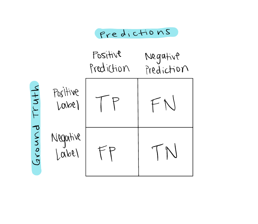
On top we have model predictions and on the side we have true labels, also known as ground truth also known as reality. If the model predicts the positive label for one sample and the sample is in fact positive, that is one True Positive. On the other hand, if the model predicts the positive label for one sample and the sample is in fact negative, that is one False Positive. And vice versa for negative samples.
Sometimes I find the idea of “positive” and “negative” labels conceptually hard to grasp because, let’s think back to our iris flower example, what makes one species the “positive” label and one species the “negative” label? I think the point is that there is one label we are more interested in than the other, like if I’m more interested in the Versicolor species than I am the Virginica species for some reason. The “positive” and “negative” labels make more conceptual sense to me in scenarios where we are predicting whether a sample has or is some ~thing~ or not, like the presence of a disease (versus no disease) or a spam email (versus a regular email). The positive label is the target event.
Here is a less generic confusion matrix tuned to our example:
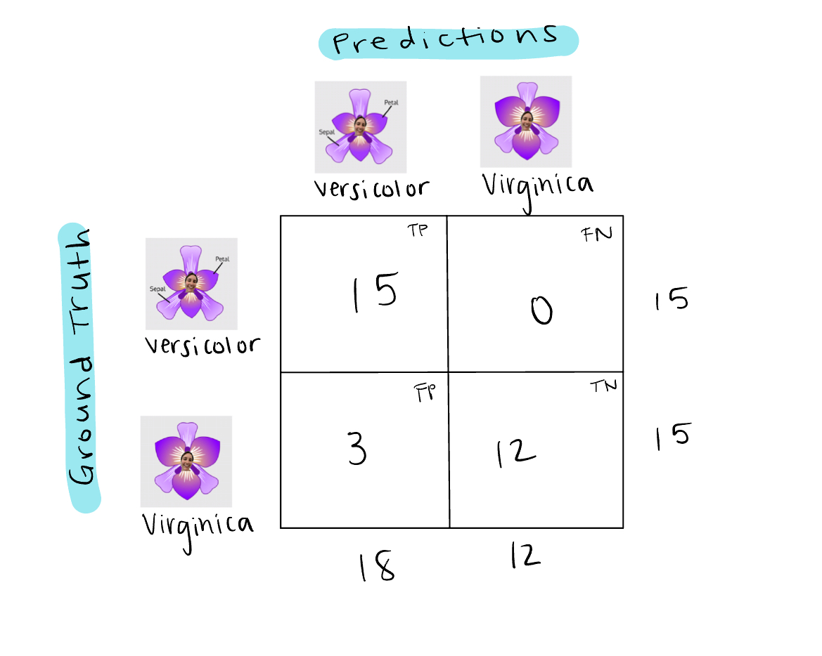
Ok so, in the test set, there are 15 Versicolor labelled flowers and 15 Virginica labelled flowers. However, the model predicts 18 Versicolor flowers and 12 Virginica flowers. It predicts all 15 Versicolor flowers correctly, but it also predicts 3 Virginica flowers as Versicolor. The formula for accuracy is
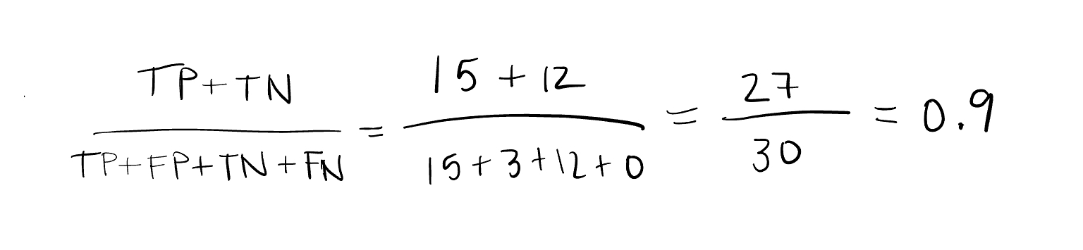
So that’s what 90% accuracy means! Accuracy is just one of many evaluation metrics used to measure how well the model is classifying ~something~. Unfortunately it’s not great for imbalanced datasets, such as in the case of rare diseases, because it can just predict the majority class and get high accuracy (2), as shown below in the case that we had way more Versicolor samples than Virginica:
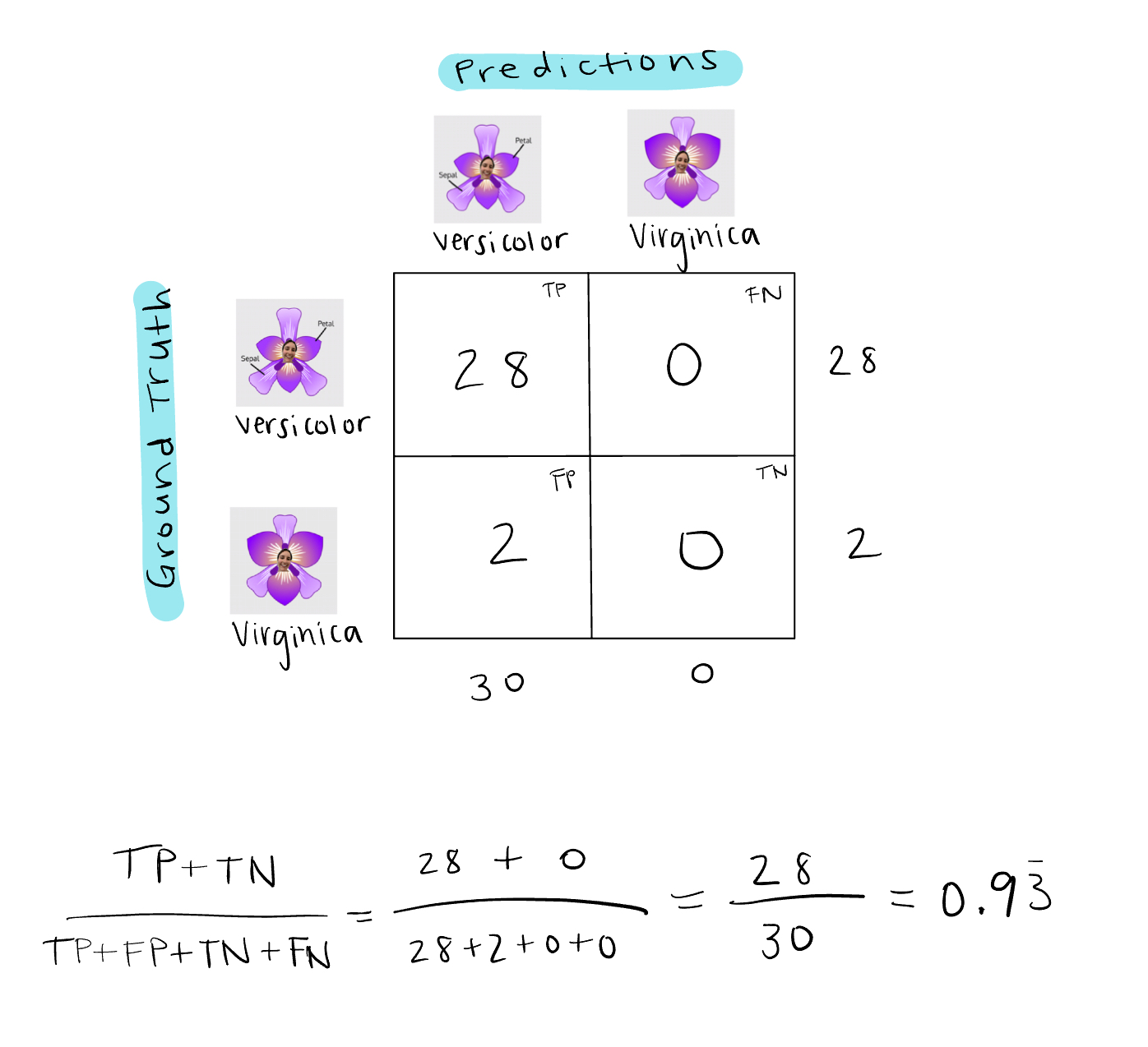
If we had 28 Versicolor samples and 2 Virginica samples and the model predicted Versicolor for every sample, accuracy would be over 90% even though it missed every Virginica sample. So much for accuracy, am I right?
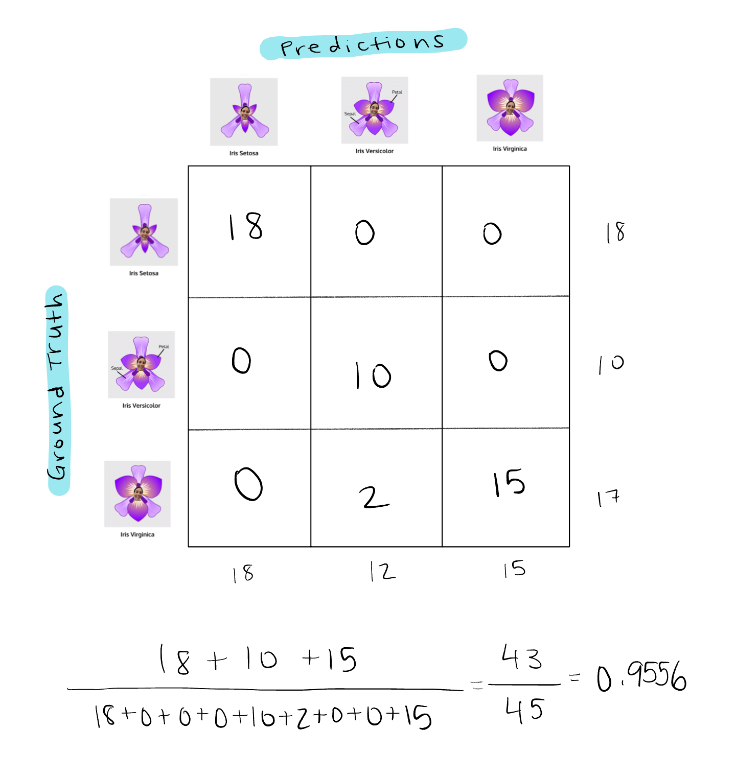
FYI, we can also use confusion matrices to get evaluation metrics for multiclass classification problems too. As the number of classes in the multiclass prediction problem increases, the dimensions of the confusion matrix grow too. Using the iris dataset again, let’s reintroduce Setosa, the third species of iris flower we removed earlier. So now, using the same model and setup as before to calculate accuracy, our confusion matrix and accuracy calculation would look something like this:
Now, let’s swivel back to binary classification. What more can we get from the confusion matrix? It’s actually chock full of useful information for evaluating model performance.
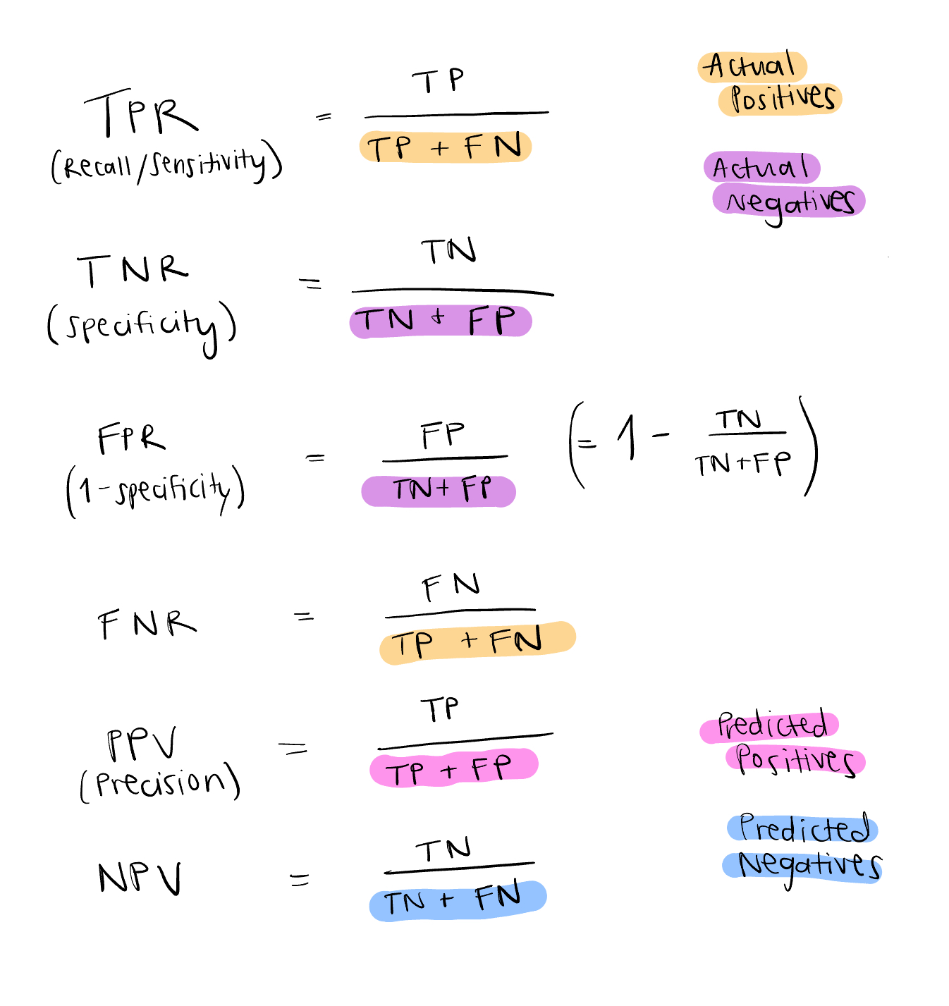
True Positive Rate (TPR), aka Recall, aka Sensitivity, is the percentage of target events the model correctly identified. Its alternate names recall and sensitivity come from different fields where TPR is also commonly utilized for evaluating performance. Recall refers to how much information was retrieved (or recalled) correctly from a query. Sensitivity comes from “sensitive” medical tests that easily show positive for presence of a disease or condition, even for people who don’t have it. (Note: I got this information from a stack exchange Q&A, but it makes sense to me).
True Negative Rate (TNR), aka Specificity, is the percentage of non-target events the model correctly identified. False Positive Rate (FPR), aka 1 - Specificity, is the percentage of non-target events the model incorrectly identifies as target events. False Negative Rate (FNR) is the percentage of target events the model incorrectly identifies as non-target events.
Precision, aka Positive Predictive Value (PPV), is the likelihood that the model accurately predicts positive values. Negative Predictive Value (NPV) is the likelihood that the model accurately predicts negative values. It’s also important to note that PPV and NPV are influenced by the presence of the target event, so if a disease is prevalent, PPV will be higher because positive predictions tend to be positive more often. Likewise for NPV and a rare disease, if the disease is not prevalent, true negatives will tend to be true more often (3).
Let’s look at some equations before we move on:
You can try these out using our binary classification example above and see the difference between your findings when you use the balanced dataset versus the imbalanced one.
Precision (PPV) values the model detecting true positives correctly at the cost of missing some positive cases, or at the cost of the model accumulating some false negatives (4). The tradeoff is that as long as the model is identifying the actual positive cases correctly, it doesn’t mind missing some. Recall (TPR) values the model detecting true positives at the cost of accumulating some false positives, so the tradeoff is that as long as it’s hitting as many true positives as possible, it doesn’t mind also including some false positives. Precision: minimize false positives. Recall: minimize false negatives.
F1 score balances precision and recall by taking a harmonic mean of the two evaluation metrics. Harmonic mean is a way to take the average of ratios, and the formula is
F1 is actually a case of the F-β function that can be reduced into the harmonic mean of precision and recall. β represents how much more we value recall over precision, so F1 means we value precision and recall equally, a lower β indicates we value precision more and a higher β indicates we value recall more (4). Here’s F-β:
And here’s F1:
We can calculate it in Python with sklearn.metrics.f1_score. When we maximize the F1 score, we are maximizing both precision and recall (6). If one or the other is too low, indicating poor model performance with either too many false positives (bad precision) or too many false negatives (bad recall), the F1 score will reflect that. An F1 score of 1 exactly indicates a perfect model, meaning no false positives nor false negatives.
Another common evaluation metric that is birthed from confusion matrix info is the Area Under the Receiver Operating Characteristic curve (AUROC), or just Area Under the Curve (AUC) . Let’s break it down, starting with the Receiver Operating Characteristic (ROC) curve. First of all, what’s the significance of its name? It was originally created by electrical and radar engineers during WWII to evaluate their radar receivers’ ability to detect enemy objects in battlefields. It could be hard to discern between actual enemy aircraft activity and noise, like clouds or birds, so they made the ROC curve to measure the sensitivity (true positive rate) of their receivers (7).
The ROC curve plots TPR (y-axis) against FPR (x-axis) at different decision thresholds. A decision threshold is the threshold at which the probabilistic classification model marks the sample as the target event. Like, if we are deciding whether an email is spam or not, a threshold at 40% means that, if the model is at least 40% certain that the email is spam, it marks it as spam. A stricter threshold would be 80%, so the model only marks the email as spam if it is 80% certain that it is spam. A lower threshold is a more lenient model that detects more false positives and a higher threshold is a stricter model that detects more false negatives. So with ROC, we graph that and try to find a threshold that has a balance between the two.
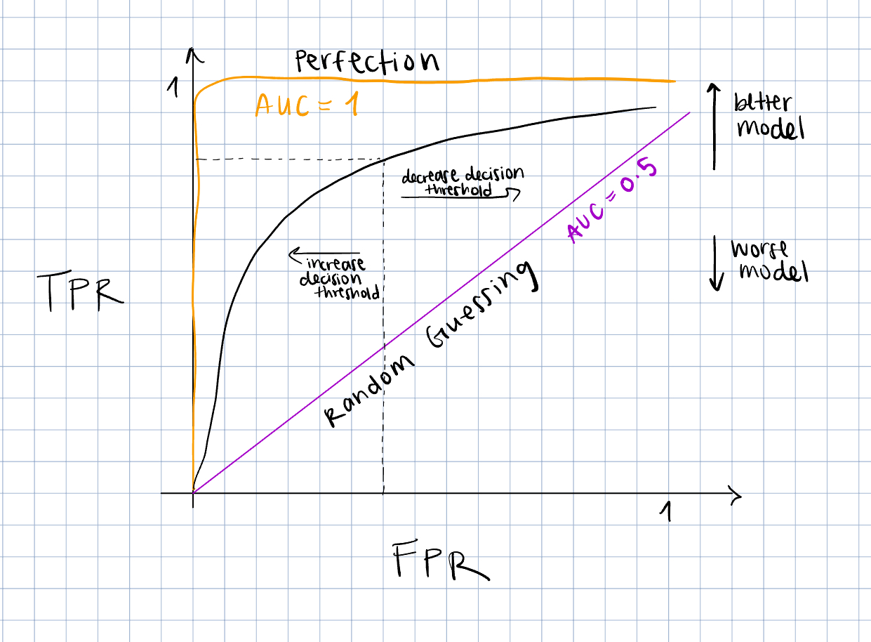
And AUROC ? Well, given a positive sample and negative sample (a target and a non-target), it tells us the probability that the classifier will give the real positive sample a higher probability of being positive than the real negative sample (8). We can compute it using the trapezoidal rule for approximating the area under a curve from calculus, or in Python with sklearn.metrics.auc (9). Up to you. Perfect AUROC is 1, indicating only true positives and no false positives, and an AUROC of 0.5 indicates that the model is as accurate as random guessing.
It’s a convenient measure of the model’s ability to predict the target event, since usually we want to increase TPR and decrease FPR, but it’s important to note that it doesn’t take into account false negatives, which can be more costly than false positives (re: missed disease diagnosis) (10). It can also be very misleading if the positive class is small. The model can predict almost every sample as negative and miss most of the true positive samples with no effect on AUROC since there are so few true positives. Enter AUPRC.
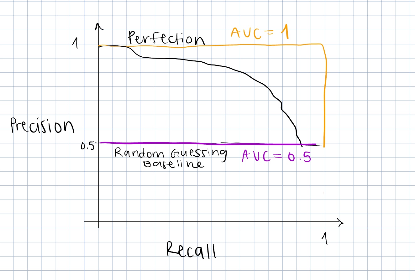
The Precision Recall Curve (PRC) plots precision (y-axis) against recall (x-axis). Area Under the Precision Recall Curve (AUPRC) works the same as AUROC, just with a different curve. It’s also available in Python with sklearn.metrics.precision_recall_curve (11). It does not consider true negatives, which is good news for an imbalanced dataset where we want to correctly predict the minority positive class (12). It also doesn’t inflate the performance of a model that only correctly predicts true negatives the way that AUROC does.
The point is, a lot of the time our dataset is going to be imbalanced with the target event as the smaller class, so we have to adjust the way we evaluate our classifiers to take that reality into account. The other point is that common, popular evaluation metrics like accuracy and AUROC can be misleading, so it’s essential to have a deeper understanding of the distribution of our dataset and what the evaluation metric we are using is measuring before feeling satisfied with our assessment of the model’s performance. The other other point is to always consider more than one evaluation metric. Look at the model’s performance from many different angles before saying anything conclusive about how well it’s doing its job. Shoutout scikit-learn giving us easy access to calculating these metrics in Python!