flavors of ice cream machine learning

Machine learning (ML) comes in many flavors, just like ice cream. Here I will describe some of them.

I initially just wanted to only focus on reinforcement learning for this post, but it seemed to make the most sense to define it within the context of other types of ML, and also knock out five birds with one stone.

* You might be wondering why deep learning isn’t included in types of machine learning. While it is a type of ML, deep learning describes the architecture of the model, while the types of ML we cover here (supervised, unsupervised, self-supervised, and reinforcement learning) are all related to the relationship between the model and its training data.

Starting with…

Supervised Learning

I would say that supervised learning is the most common type of ML that we hear about. Essentially, it refers to a machine learning model trained on a labeled dataset. Example algorithms include: logistic regression, support vector machines (SVM), decision trees, and neural networks. It is used for regression and classification tasks and we can measure the results from the model against the ground truth that the labeled data provides us. Pretty chill, in the sense that we have fully labeled data to train the model on. It is useful in any domain that has labeled data available, so maybe things like image classification, like labeling apples versus oranges, and so on.

Unsupervised Learning

Unsupervised learning refers to a model that uncovers patterns in unlabeled data that may not even be apparent to humans. It does not measure results against a ground truth, as there is no ground truth provided. Some algorithms include: k-means, principal component analysis (PCA), hierarchical clustering, and anomaly detection. Essentially, it outputs data organized in groups with each group’s characteristics. Useful for things like fraud detection, where it finds the data that differs from the rest, or recommendation systems, where it identifies patterns in the data which it then uses to recommend stuff.

Okay, so: supervised learning uses labeled data, unsupervised learning doesn’t. Got it. Now this is where things start to get a little bit sticky…

Self-supervised Learning

Self-supervised learning (SSL) uses unsupervised learning for tasks that normally require supervised learning. Note that, all SSL is unsupervised learning, but not all unsupervised learning is SSL. First step is pretext learning, where the model gives the unlabeled data “psuedo-labels”, thereby sort of creating a ground truth which it uses to measure results against. It replaces the need to manually label data, which is particularly useful for computer vision and natural language processing (NLP) tasks, where there are massive amounts of unlabeled data available while the tasks require massive amounts of labeled data. Other than using unlabeled data, SSL is more similar to supervised-learning in that it refers to a ground truth and is used for classification and regression.

There are two types of SSL, or two ways the model goes about predicting labels: self-predictive and contrastive.

Self-predictive learning

Also known as autoassociative SL or generative SL, self-predictive learning essentially predicts one part of the data from another. Some examples of self-predictive learning include:

Autoencoders are neural networks that encode and then decode the data.

Autoregression is a model that uses past data to predict future data, based on the idea that any data with a sequential order can be predicted using regression. (What is regression, really? Well, there are a few different types, but the basic idea is just understanding the relationship between a target variable (output) and other features (input) and then using that relationship to predict future instances of the target.)

Masking is covering a part of the unlabeled data and predicting it based on surrounding data as context. Its glory is in the fact that it works bidirectionally, so it captures different, more complex relationships between the data as it looks at it from multiple angles. A common example of a masking model is BERT.

Contrastive learning

Contrastive learning predicts the relationships between data samples It is known as a discriminative method because it learns to distinguish between similar and different samples. Some examples of self-predictive learning include:

Instance discrimination takes one sample as the target and learns to determine whether other samples are similar to or different from it. Using the help of data augmentation for creating new instances of data, it is also robust to small variations in samples, such as a different color or rotation.

While contrastive learning usually compares positive data samples against negative ones, non-contrastive learning only considers positive data samples and focuses on reducing the difference between two augmented views of the same sample. By completely omitting negative samples, non-contrastive learning requires less samples while maintaining comparably good results.

Multi-modal learning learns to identify similarities between different types of data. For example, matching text labels to images.

After psuedo-label creation comes the downstream classification/regression task, which brings us to semi-supervised learning. Semi-supervised learning uses a small amount of labeled data to finetune the model for a specific task. This is necessary because the pseudo-labeling gives the model a general understanding of the dataset, but fine-tuning to a chosen task improves accuracy and the model’s understanding. So, semi-supervised learning uses a combination of labeled and unlabeled data to train the model.

Self-supervised learning and semi-supervised learning are separate entities, but are often combined for optimal results. The point is, we started with an unlabled dataset and, using self-supervised and semi-supervised learning, we got a labeled datset that can now be used to train models for tasks normally delegated to supervised learning models. Cool!

Okay now here comes the big tuna:

Reinforcement Learning

Using reinforcement learning (RL), the model aims to mimic real-world biological learning methods by learning through rewards and penalties. Actions that have led the model to a reward are reinforced (shocking). It is best used in areas that can be fully simulated. Self-driving cars are a typical example of RL. After you finish this section, maybe you’ll have a better idea about how those Waymos were trained the next time you see one in the Bay Area. It's also amazing at games like chess, since it can spend many more hours playing against itself and improving its performance than a human realistically can. RL does not use labeled data, but it is not considered an unsupervised learning method because of the reward-punishment system it uses which makes it unique from other learning types.

Here's a quick visual example:

Okay while I enjoy that ice cream, let’s delve a little deeper into how it actually works.

There’s a few components involved:

The autonomous agent, or the decision-maker performing the action who can make decisions without direct interaction from humans. The environment, or the world/system that the agent operates in. The state, or the situation the agent is currently in. The action, or the possible decision the agent can make. The reward/punishment, or the feedback from the environment based on the agent’s chosen action.

More components that are integral to the process:

The policy defines the agent’s behavior by mapping states to actions that agents should take in those states; it is updated based on the received feedback. While the reward signal is the goal of the problem and the immediate feedback about the utility of an action in that moment, the value function takes into account more long-term benefits; it measures the desirability of an action considering future outcomes. (Imagine a soccer-playing agent that gets an immediate reward for touching the ball, so it kicks the ball back and forth to itself to increase immediate rewards in the short term, but loses focus on the overall objective of scoring goals. Over time, it will realize the total value function is larger when it moves the ball toward the goal and replace reward-farming for a greater long-term purpose). The model is an optional component that allows agents to predict environmental behavior for possible actions (i.e. predicting the behavior of surrounding vehicles).

Like I mentioned before, actions that result in a reward are reinforced, but the agent can’t solely perform the same actions that have garnered rewards. The agent must continue to explore the environment by trying new actions, so there must be a balance between exploiting knowledge from previously rewarded actions and trying new ones.

The general RL cycle goes like this:

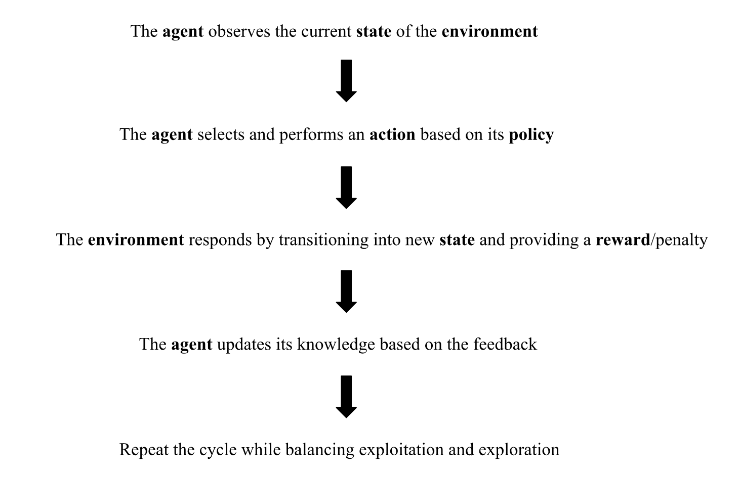
This cyclical way of describing the RL pipeline is based on the Markov Decision Process (MDP). Briefly put, MDP is a mathematical framework for decision-making in uncertain scenarios which assumes that the current state provides all necessary information for coming to an optimal decision.

RL can function online, collecting data and processing it iteratively as the agent interacts with the environment, or offline, without direct access to an environment and with the agent learning from logged data.

There are also different types of RL. Hooray. Honestly, I’m not going to go into them here because I think each one could take up a blog post of its own. But just so you know, there’s Dynamic Programming, Monte Carlo method, Temporal Difference learning (which includes well-known algorithms Q-learning and SARSA), Policy Gradient method, and Actor-critic method.

So overall, RL is cool because it can solve complex sequential problems and adapt to changing environments. BUT, it’s computationally intensive, an optimal reward function is essential yet infamously challenging to figure out, and it doesn’t work well for simple problems.

That was fun. Thanks for reading.

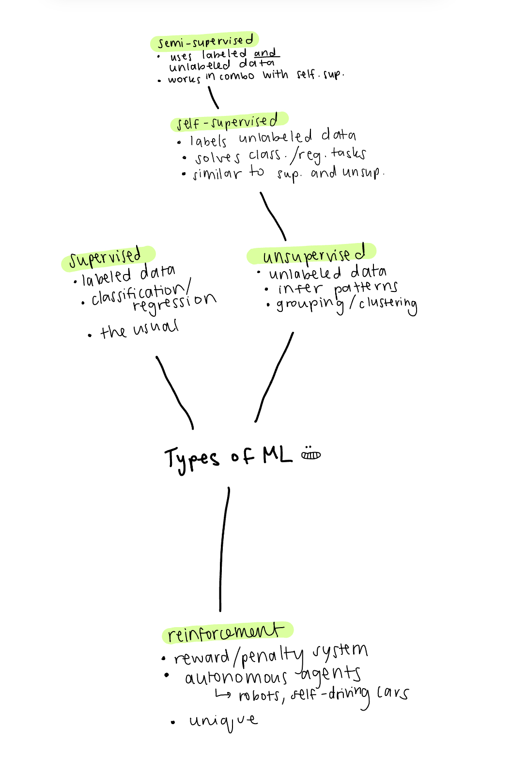
Here's a little summary mind map I made: